1. Measuring a network
In this chapter
You will learn
- why a production fabric needs continuous, active measurement in addition to SNMP, syslog and ping
- where the delay of a packet comes from - serialisation, propagation, processing and queuing - and how large each part is on the LVR paths
- why one-way delay normally needs synchronised clocks, and why TRex does not
- the difference between the "jitter" that TRex reports (RFC 3550) and packet delay variation (RFC 5481)
- how loss is counted, what the loss resolution of a stream is and how to turn lost packets into an outage duration
- how to summarise latency honestly (minimum, average, maximum, histogram) and why the maximum matters
- the benchmarking vocabulary you will meet in test reports (RFC 2544 throughput, NDR, back-to-back, IMIX)
Prerequisites: none
Every number on the LVR dashboards is one of a handful of measurement quantities: one-way latency, jitter, loss, reordering and duplicates. They look simple, but each has a precise definition, a resolution and a set of traps. As the support person for the platform you will be asked questions such as "Grafana shows 180 µs between Kalk and Chorweiler - is that bad?" or "there was a 40 ms outage during the firewall failover - how sure are we?". This chapter gives you the vocabulary and the arithmetic to answer them. It needs no TRex knowledge; the TRex mechanics follow in chapter 4 and chapter 5.
Why measure continuously
A data-centre fabric rarely fails cleanly. Links that go down, routing adjacencies that drop and devices that reboot are visible immediately in syslog, SNMP traps and the routing table - and the fabric usually routes around them. The failures that hurt users are the ones the control plane does not see. They are called grey failures (in the literature usually "gray failure"):
- An optic slowly degrades and one member of a link aggregation or one ECMP path starts dropping a fraction of a percent of the frames hashed to it. OSPF, BGP and LACP stay up; every device reports "healthy".
- A forwarding problem in one IRF member affects only one VLAN or one VXLAN tunnel.
- A firewall cluster member under load still forwards everything, but adds hundreds of microseconds.
- A MAC address keeps moving between two ports, and for a few hundred milliseconds at a time traffic goes the wrong way.
Health monitoring (interface up/down, CPU, memory, syslog) answers the question "are the devices alive?". Active measurement with synthetic traffic answers a different question: "does a packet that enters here leave there, how long does it take, and does it arrive intact and in order?". That is the question users ask.
Continuous measurement adds three things that ad hoc tests cannot provide:
Change validation. A software upgrade (for example of SW-RZC-L21, which still runs R6205P03 while the other
examined switches run R6301 or later), a firewall policy installation or a new DCI optic can be judged by comparing the
same streams before and after. Without a permanent measurement you are comparing against memory.
Baselines. "Is 38 µs a lot?" has no answer in isolation. A stream whose minimum has been 37 µs for months and whose maximum suddenly jumps to 400 µs tells a clear story. The baseline is what turns a number into information.
Evidence. Service levels - formal or informal - need numbers. When an application team reports "the network is slow", per-path latency and loss for the time in question either show a network problem or rule it out.
In the LVR platform
The running configurations show that measurements have been done before, ad hoc: a QoS policy iperf-counting
(classifier iperf-5001 matching UDP destination port 5001, behaviour packet-counter) is applied inbound on
Route-Aggregation1 (the DCI) of both Border Leafs and on Bridge-Aggregation31 (the DC firewall channel) of
sw-rzk-BL, and port FGE1/4/26 of sw-rzk-BL is labelled "ALLEGRO-TEST". The TRex platform turns such one-off
tests into permanent, comparable measurements that do not depend on someone remembering to run iperf.
Where delay comes from
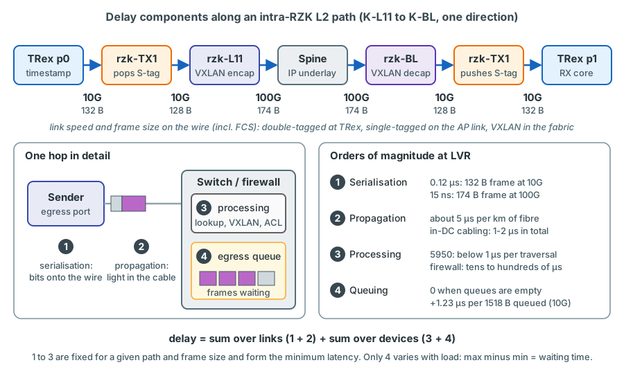
A packet travelling from A to B crosses a series of links and devices. Its delay is the sum of four kinds of contribution, added up over every hop:
delay = sum over all links    ( serialisation + propagation )
      + sum over all devices  ( processing + queuing )
The first three are essentially fixed for a given path and frame size. Queuing is the variable part - and the part that tells you about congestion.
Serialisation
Serialisation delay is the time it takes to clock the bits of a frame onto the wire:
On Ethernet a frame occupies more of the wire than its own length. Before every frame the sender transmits a 7-byte preamble and a 1-byte start-of-frame delimiter, and after it the line must stay idle for at least 12 bytes (the inter-frame gap). Together that is 20 bytes per frame that carry no data but occupy the link. The 4-byte frame check sequence (FCS) is part of the frame itself.
Be careful with frame-size conventions. The classic benchmark sizes (64 and 1518 bytes) include the FCS. TRex packet sizes exclude it, because the NIC appends the FCS in hardware: the LVR monitoring frame is configured as 128 bytes in TRex and therefore leaves the NIC as a 132-byte frame.
| Frame size (incl. FCS) | On the wire incl. 20 B preamble/SFD/gap | 10 Gbit/s | 40 Gbit/s | 100 Gbit/s | Max. frames/s at 10G |
|---|---|---|---|---|---|
| 64 B (minimum) | 84 B = 672 bit | 67.2 ns | 16.8 ns | 6.7 ns | 14.88 million |
| 128 B | 148 B = 1 184 bit | 118.4 ns | 29.6 ns | 11.8 ns | 8.45 million |
| 132 B (LVR monitoring frame, 128 B in TRex) | 152 B = 1 216 bit | 121.6 ns | 30.4 ns | 12.2 ns | 8.22 million |
| 1518 B (maximum untagged) | 1 538 B = 12 304 bit | 1 230.4 ns | 307.6 ns | 123.0 ns | 0.81 million |
The right-hand column follows from the same arithmetic: at 10 Gbit/s a new 64-byte frame can start every 67.2 ns, so the line rate is 10 000 000 000 / 672 = 14.88 million frames per second. You will meet this number again in chapter 3, because it defines the time budget a traffic generator has per packet.
Two remarks put the table into perspective:
- For the maximum frame rate the full 20 bytes count. For the delay a store-and-forward hop adds, only the preamble, delimiter and frame count (the gap follows the frame); for small frames that is about 10 % less. At the scale of the LVR measurements the difference does not matter.
- A frame changes size along the path. The LVR monitoring frame is double-tagged between TRex and the TX switch (132 bytes), single-tagged on the attachment link to the Leaf (128 bytes) and VXLAN-encapsulated in the fabric: the Leaf removes the remaining VLAN tag and adds 50 bytes of outer headers (Ethernet, IPv4, UDP, VXLAN), giving 174 bytes on the wire. On the 100 Gbit/s Leaf-Spine links even that takes only about 15 ns.
In the LVR platform
The Leaf-Spine links are 100G: display interface in the diag file of sw-rzk-L11 shows HundredGigE1/1/3
("-> Link to Spine1") in "100Gbps-speed mode, full-duplex mode" with a 100G AOC. The attachment points and the
TRex ports are 10G, and the DCI between the Border Leafs is 2 x 40G. On the path of an intra-DC monitoring stream the
serialisation delays add up to about half a microsecond - negligible compared with the other components.
Propagation
Light travels through glass fibre at roughly two thirds of its speed in vacuum (refractive index about 1.47), i.e. about 204 000 km/s. The rule of thumb you should remember is:
propagation in fibre ≈ 5 µs per kilometre (more precisely about 4.9 µs/km)
Inside a data centre this is small: a 3 m DAC costs about 15 ns, a 100 m fibre run 0.5 µs. Between data centres it
dominates everything else. The DCI between sw-rzk-BL and sw-rzc-BL uses 40G ER4 optics (a 40 km class), which
suggests a fibre path longer than 10 km; the real distance still has to be confirmed. If the path were 15 km long
(an illustrative value), a single crossing would add 75 µs - more than all switches of a data centre together.
Processing: switching, routing, firewalls
Every device spends time deciding what to do with a frame: parsing headers, looking up the MAC or IP table, applying ACLs and QoS, adding or removing a VXLAN header. Two forwarding principles matter:
- A store-and-forward device receives the complete frame, checks the FCS and only then starts transmitting. It adds at least the serialisation time of the frame at every hop.
- A cut-through device starts transmitting as soon as it has read enough of the header to make the forwarding decision. It saves most of the serialisation time but forwards corrupted frames it cannot yet recognise. A switch typically falls back to store-and-forward when the egress port is faster than the ingress port or is busy.
The HPE FlexFabric 5950 is a cut-through design. HPE specifies its latency as below 1 µs at 10 Gbit/s for 64-byte packets (QuickSpecs, also for the 4-slot model JH404A used as Leaf and Border Leaf at LVR). VXLAN encapsulation on the ingress Leaf, decapsulation on the egress Leaf and routing on the Border Leaf happen in the same forwarding pipeline; you should expect each switch traversal to cost around a microsecond, not tens of microseconds.
Firewalls are different. A stateful firewall looks up (or creates) a session for every packet, applies the rule base, possibly NAT and inspection, and runs at least part of this work in software. Its forwarding delay is typically tens to hundreds of microseconds and depends on load, on the features that inspect the flow and on which cluster member is active. The LVR classes that cross the DC firewall or the Enterprise firewall will therefore show both higher and more variable latency than the pure fabric classes.
Queuing - the variable part
When a frame arrives at an egress port that is already transmitting, it waits in a queue. Every 1518-byte frame ahead of it in the queue of a 10G port adds 1.23 µs; one hundred such frames add 123 µs. Queues build up during microbursts - several ports sending to the same egress port at the same moment - even when the average utilisation over a minute is low. The 5950 has a 16 MB packet buffer (QuickSpecs), enough to hold frames for many milliseconds when congestion is severe.
Queuing is the reason latency is such a good health indicator. In an idle network the queues are empty and a stream's latency sits at its minimum: the fixed part made of serialisation, propagation and processing. Everything above the minimum is, to a first approximation, waiting time in queues - or extra processing in a device that is struggling.
Worked example: delay budget of an intra-RZK stream
The table estimates the one-way delay of an L2 monitoring stream from attachment point K-L11 to K-BL in VLAN 1314. The values are planning estimates, not measurements illustrative values.
| Contribution | Basis of the estimate | Estimate |
|---|---|---|
| Serialisation | 6 transmissions: TRex→TX1, TX1→L11, L11→Spine, Spine→BL, BL→TX1, TX1→TRex (4 x 10G, 2 x 100G) | ≈ 0.5 µs |
| Propagation | about 300 m of DAC and fibre in total (assumed) | ≈ 1.5 µs |
| Switch processing | 5 traversals (TX1, L11, Spine, BL, TX1), each below about 1 µs | < 5 µs |
| Queuing | empty queues in normal operation | ≈ 0 |
| TRex's own share | time from writing the TX timestamp to processing the packet on receive (software mode) | a few µs in the one-queue receive model that trex-mon uses; up to about 20 µs more in the multi-queue model (chapter 3); measured in the loopback test |
The network part comes to well under ten microseconds; the measured value adds TRex's own share. The planning value used throughout the course is "up to a few tens of microseconds" for intra-DC fabric paths. The baseline measured after bring-up replaces all such estimates.
One-way delay, round-trip time and the clock problem
What ping really measures
ping measures the round-trip time (RTT): forward delay plus the responder's processing time plus the reverse
delay. That has three consequences that matter in a fabric:
- The responder is a CPU, not a forwarding pipeline. When you ping the gateway 10.3.14.1 on
sw-rzk-BL, the ICMP echo reply is generated by the switch's control-plane processor. That path is rate-limited and scheduled behind routing protocols; it tells you how busy the switch CPU is, not how fast the ASIC forwards. - Asymmetry is invisible. An RTT of 400 µs could be 200 + 200 or 50 + 350. At LVR, asymmetric paths are normal: routed traffic from Chorweiler crosses the DCI to its gateway in Kalk, and the path through a firewall cluster depends on which member is active. Only one-way measurement shows which direction is slow.
- Resolution is coarse. ping reports milliseconds or tenths of milliseconds; fabric paths take a few to a few tens of microseconds.
One-way delay needs two clocks - normally
To measure one-way delay, the sender writes its transmit time into the packet and the receiver subtracts it from its receive time. If sender and receiver are different machines, the result is:
RFC 7679, which defines the IETF one-way delay metric, lists the clock properties that limit such a measurement: synchronisation (how far two clocks disagree - its example is a clock 5.4 ms ahead of another), accuracy (how far a clock is from UTC), resolution (the smallest step of the clock) and skew (how fast the offset changes). With NTP, servers typically agree to within a fraction of a millisecond up to a few milliseconds - far too coarse for fabric paths of a few to a few tens of microseconds, where the offset error would be larger than the quantity you want to measure. PTP with hardware time-stamping can reach sub-microsecond agreement, but needs a timing infrastructure (grandmaster, PTP-aware network or careful design, time-stamping NICs at both ends).
The TRex way: one clock, a loop through the network
TRex sidesteps the problem completely: the transmitting and the receiving port are in the same server and read the same clock. When a data-plane core sends a latency packet, it writes a 16-byte trailer into the last bytes of the payload: an internal stream index, a per-stream sequence number and a 64-bit transmit timestamp taken from the CPU's time-stamp counter (TSC). When the packet comes back in on another port, the TRex core that receives it reads the trailer and subtracts the timestamp from the current TSC value. Offset and skew between "sender" and "receiver" are zero by construction; the counter ticks at the CPU clock rate, so the resolution is far below a nanosecond. What limits the accuracy is the software path inside TRex, which is why the TRex documentation describes its latency measurement as "microsecond resolution (software-based)", in contrast to the nanosecond, hardware-based timestamps of commercial testers.
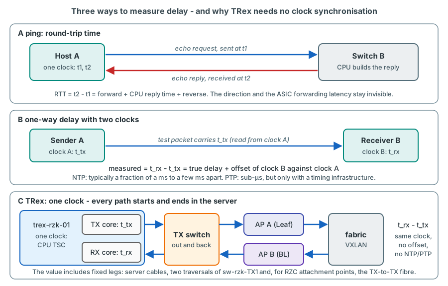
The price is topological: every measured path must start and end at the TRex server. At LVR the server stands in
Kalk, and the attachment points in Chorweiler are reached over the dedicated TX-to-TX fibre between sw-rzk-TX1 and
sw-rzc-TX1. A "one-way" value is therefore always the path from attachment point A to attachment point B plus fixed
measurement legs: the server-to-TX-switch cables, two traversals of sw-rzk-TX1 and, for Chorweiler attachment points,
sw-rzc-TX1 and the TX-to-TX fibre.
| Stream direction | TX-to-TX fibre crossings | Where |
|---|---|---|
| RZK → RZK | 0 | - |
| RZK → RZC | 1 | on the way back to the server |
| RZC → RZK | 1 | on the way out from the server |
| RZC → RZC | 2 | out and back |
With an (illustrative) 15 km TX-to-TX fibre, an intra-RZC stream would show about 150 µs more than the same kind of
stream inside RZK, even if both fabrics were identical. An inter-DC L2 stream additionally crosses the DCI once in the
direction it measures; a routed stream between two Chorweiler attachment points crosses the DCI twice, and one between a
Chorweiler and a Kalk attachment point once, because its gateway is on sw-rzk-BL in Kalk.
Why not subtract the fibre delay automatically?
Because the subtraction itself would need a measurement that can drift. The platform reports absolute values and
documents the fixed offsets separately. The fibre offset is calibrated by comparing the same stream type inside RZK
and inside RZC: the difference is twice the one-way TX-fibre delay plus the two extra traversals of sw-rzc-TX1.
Dashboards can show the offset as a reference line, but the raw number stays raw. Chapter 16
and the animation in chapter 14 go into the details.
Jitter and delay variation
"Jitter" is used loosely for anything that makes delay unsteady. The IETF distinguishes two precise forms of delay variation, and TRex reports a third, smoothed quantity. You need to know all three to read the dashboards correctly.
Two definitions of delay variation (RFC 5481)
Let D(i) be the one-way delay of packet i of a stream.
- IPDV - inter-packet delay variation:
IPDV(i) = D(i) - D(i-1), the change of delay from one packet to the next. It can be positive or negative and its mean over a stable stream is about zero. - PDV - packet delay variation:
PDV(i) = D(i) - D(min), the delay of each packet above the smallest delay seen in the measurement interval. It is never negative.
RFC 5481 illustrates the difference with five packets (values in ms):
| Packet | 1 | 2 | 3 | 4 | 5 |
|---|---|---|---|---|---|
| Delay | 20 | 10 | 20 | 25 | 20 |
| IPDV | undefined | -10 | +10 | +5 | -5 |
| PDV | 10 | 0 | 10 | 15 | 10 |
PDV is the delay distribution shifted to zero. Its percentiles have a physical meaning ("99.9 % of the packets arrived less than 15 ms above the fastest one"), which is why RFC 5481 recommends PDV, for example its 99.9th percentile, when a single number is needed for a service level. IPDV is two-sided and depends on the order of the packets; it is preferred when paths change often or clocks drift, but it does not summarise well.
What TRex reports: RFC 3550 interarrival jitter
The jitter value TRex reports per latency stream is the interarrival jitter of RTP (RFC 3550, section 6.4.1 and
appendix A.8). For every received packet:
transit(i) = receive time - transmit timestamp          (the one-way delay of packet i)
D          = transit(i) - transit(i-1)                   (an IPDV value)
J          = J + ( |D| - J ) / 16                        (exponential smoothing)
TRex implements exactly this estimator (trex-core src/utils/utl_jitter.h) on its one-way transit times. In plain
words: TRex jitter is a smoothed average of how much the delay changes from one packet to the next. The factor 1/16
gives it a memory of roughly 16 packets - about 80 ms at 200 pps, 320 ms at 50 pps.
This has consequences you must keep in mind:
- A stream with a high but constant delay has a jitter of zero. Jitter says nothing about the delay itself.
- A single spike is strongly damped. If one packet out of a steady 20 µs stream is delayed to 120 µs, D is +100 µs for that packet and -100 µs for the next; J rises only to about 12 µs and then decays.
- A slow change - a queue that fills over several seconds - hardly moves J at all, because consecutive packets see almost the same delay.
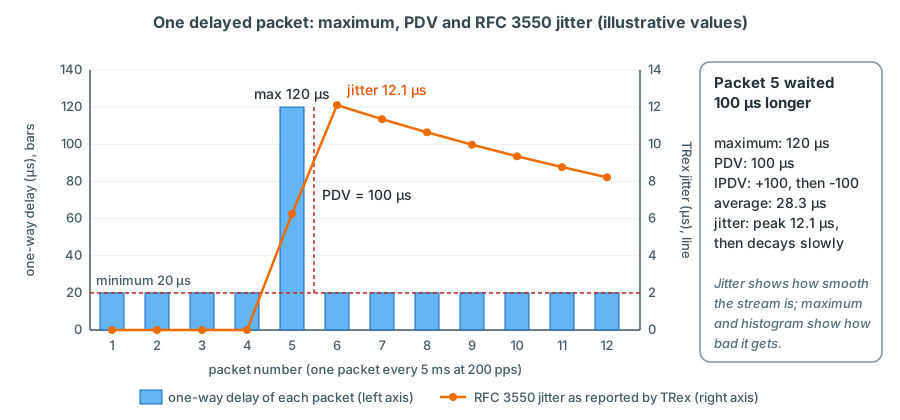
Use the measures for what they are good at: jitter answers "how smooth is this stream at the moment?", the maximum and the histogram (a PDV view: delay above the minimum) answer "how bad does it get?". The LVR dashboards show both. Chapter 5 explains how the TRex statistics are sampled.
Packet loss
Counting loss: two methods
TRex offers two ways of detecting loss, and the LVR monitoring profile uses both.
Counter-based loss. Every stream that carries a packet group ID (pg_id) is counted on transmit and on receive.
Loss over an interval is simply TX packets - RX packets. This works for any rate and is cheap, which is why the LVR
loss-only streams (flow-stat streams) use it. Its limits: the counters are read periodically, a few packets are always
in flight, and transmit and receive counters are not sampled at exactly the same instant - a difference of one packet
that disappears in the next interval is a sampling effect, not loss.
Sequence-based loss. Latency streams carry a sequence number in their 16-byte trailer. The receiver knows which
number it expects next; a jump forward means packets were lost, a number that is too low means a packet came late
(reordering) or twice (duplicate). TRex keeps counters for these events - dropped, out_of_order, dup,
seq_too_high and seq_too_low - and explains in its API documentation that dropped, dup and out_of_order are
heuristics derived from the sequence numbers (for example, a later "too low" packet decrements dropped again because
the packet thought lost has arrived after all).
Resolution and outage duration
A stream sends one packet every 1/pps seconds. That interval is its loss resolution: the smallest outage it can
quantify. If N consecutive packets are lost, the outage lasted approximately
The uncertainty of this estimate is about plus or minus one packet interval.
| Stream rate | Packet interval = resolution | Used at LVR for |
|---|---|---|
| 50 pps | 20 ms | latency streams through firewalls |
| 100 pps | 10 ms | loss-only streams; DSCP class (L2) |
| 200 pps | 5 ms | latency streams in the fabric |
| 1000 pps | 1 ms | temporary, for convergence tests |
Worked examples:
- A fabric latency stream at 200 pps loses 37 packets during an IRF member reboot: the outage lasted about 37 / 200 = 0.185 s = 185 ms, more precisely between 180 and 190 ms.
- The same event measured with a stream raised to 1000 pps loses 186 packets: 186 ms ± 1 ms.
- A firewall-class stream at 50 pps loses 9 packets during a cluster failover: 180 ms ± 20 ms.
Because each direction is a separate stream with its own pg_id, the two directions are measured independently; an outage of 185 ms in one direction and 60 ms in the other is a real and useful observation (one direction reconverged faster).
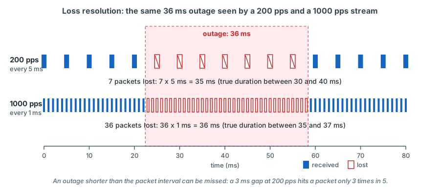
The resolution also limits what you can see at all. An outage of 3 ms on a 200 pps stream hits a packet with a probability of 3/5 = 60 %; in the other cases the stream does not notice it. If short events matter - during a maintenance window, for example - raise the rate of the affected streams for that time (chapter 23).
Why not run every stream at 1000 pps?
Higher rates cost something. Latency streams are processed in software on the TRex server and are limited to 128 per instance; every stream through a firewall creates a session and load on the firewall; and every packet crosses production links. The LVR profile therefore uses 200 pps in the fabric (5 ms), 50 pps through firewalls (20 ms) and 100 pps for the loss-only streams (10 ms), and raises rates only temporarily. Chapter 16 derives the complete budget.
Reordering and duplicates
A single stream with a fixed 5-tuple is hashed onto one ECMP path and one LAG member, so in steady state its packets
arrive in order. Reordering therefore points to a moment in which packets of the same stream took different paths:
a path change during reconvergence, a rehash after a link failure, or a load-balancing problem. RFC 4737 defines
reordering metrics; TRex counts the events (out_of_order, seq_too_low).
A duplicate - the same sequence number received twice - means the network delivered a packet more than once. In a switched network that happens when frames are flooded and reach the receiver over more than one way, or during a transient Layer 2 loop.
In the LVR platform
The monitoring ports of TRex receive every S-VLAN of every attachment point. If a destination MAC address is not known in the fabric, the Leaf floods the frame to all ports of the VSI, including every attachment point that carries this VLAN - and each of them hands a copy back to TRex. A burst of duplicates on many streams at the same time, or a flow-stat stream that suddenly receives more packets than it sent, is therefore the expected signature of unknown-unicast flooding (to be confirmed on the bench). Chapter 24 explains why flooding also matters for production safety.
Summarising latency: statistics
A latency stream at 200 pps produces 17.3 million samples a day. Dashboards must summarise them, and every summary hides something:
| Statistic | What it represents | What it hides |
|---|---|---|
| Minimum | The fixed part of the path: propagation, serialisation, processing with empty queues. Changes only when the path changes (for example a firewall failover to the other data centre) | Everything that varies |
| Average | The typical delay | Spikes: they are diluted by thousands of normal samples |
| Maximum | The worst packet in the interval: microbursts, stalls, buffer build-up | How often it happened |
| Histogram / percentiles | The distribution: how many packets fell into which delay range | Exact values within a bucket |
Why the maximum matters: take a 2-second interval of a 200 pps stream - 400 packets. If 399 packets need 20 µs and one packet is stuck for 5 ms, the average is (399 x 20 + 5000) / 400 = 32.5 µs - barely different from normal - while the maximum is 5 000 µs. A storage or VoIP session would have noticed that packet; the average does not.
TRex keeps, per latency stream, the minimum and maximum over the stream's lifetime, the maximum of the last sampling window (0.5 s), a logarithmic histogram (10 µs steps up to 100 µs, 100 µs steps up to 1 ms and so on; everything below 10 µs is counted in one bucket) and an average. The average is low-pass filtered - each sampling period the new value is half the previous average plus half the average of the last period - so it reacts within a second or two but is not a plain arithmetic mean. The consequences for an exporter that polls every few seconds are explained in chapter 5.
Active and passive monitoring compared
| Method | Type | What it tells you | Strengths | Weaknesses |
|---|---|---|---|---|
| ping (ICMP echo), NQA ICMP echo | Active | Reachability, round-trip time | Available everywhere, no setup | RTT only; the responder is a CPU; rate-limited; hides asymmetry; ms resolution |
| iperf / iperf3 | Active, between two hosts | Throughput; for UDP also loss and jitter | Simple; shows real TCP behaviour | Needs an end host per VLAN; kernel network stack limits small-packet rates; no one-way delay without synchronised clocks; ad hoc |
| SNMP interface counters | Passive | Octets, errors and discards per interface | Already in place; long history | Per device, not per path; 1-5 minute averages hide bursts; no latency |
| sFlow / NetFlow / IPFIX | Passive, sampled or per flow | Who talks to whom, volumes, top talkers | Visibility of real user traffic | Sampling; no per-path latency or loss; export delay |
| TRex synthetic streams | Active, dedicated generator | Per-path one-way latency, jitter, loss, reordering, duplicates; continuously, both directions | µs and ms resolution; deterministic; independent of user traffic | Measures only the paths you configure; needs dedicated infrastructure; adds a small load; must be operated safely |
The methods complement each other. TRex tells you that and where a path degrades - between which attachment points, in which direction, from which second. SNMP counters, sFlow and the switch logs then help you find why.
In the LVR platform
sw-rzk-BL already runs Comware NQA operations: nqa entry imclinktopologypleaseignore ping (type icmp-echo
towards 10.9.0.21, frequency 270000 - one probe every 270 s, the unit is milliseconds) and a type voice
operation named voice_dci_test. Such probes are useful for reachability and coarse trends; they cannot replace
per-path one-way measurements at microsecond resolution.
Measuring the measurement system
Every measurement includes the measuring instrument. Before you trust a value, you must know what the instrument itself contributes - and you must re-check it whenever the instrument changes. For the LVR platform that means three calibration steps:
- Loopback baseline. Two TRex ports connected directly with a DAC, no switch in between. Whatever latency TRex
reports now is its own share: the time from writing the transmit timestamp to processing the packet on the
receiving core, plus two NIC passes and one cable. It is measured during the acceptance test of the server
(chapter 17); expect a few microseconds in the one-queue receive model that
trex-monuses, and up to about 20 µs more if TRex ran in its multi-queue model (chapter 3) confirm on the bench. - TX switch share. The same test through
sw-rzk-TX1only, before attachment points are connected, adds one switch traversal. Every monitoring stream crossessw-rzk-TX1twice. - Fibre offset. Compare the same stream type inside RZK and inside RZC. The difference is twice the one-way delay
of the TX-to-TX fibre plus two traversals of
sw-rzc-TX1.
Record these values as part of the baseline and repeat the loopback test after changes to the server: a new TRex release, BIOS or kernel changes, a different core layout. Otherwise a change of the instrument looks like a change of the network.
In the LVR platform
The NQA voice operation voice_dci_test on sw-rzk-BL illustrates why validating a measurement matters: its
configured destination is 172.31.0.254, which is the Loopback0 address of sw-rzk-BL itself (the NQA server with
UDP port 9001 is configured on sw-rzc-BL, 172.31.1.254). As configured, the probe does not cross the DCI its name
refers to. A calibration step would have revealed this immediately.
Benchmarking vocabulary: RFC 2544 and IMIX
Lab tests on the platform use the vocabulary of RFC 1242 (terminology) and RFC 2544 (methodology), originally written for testing a single device under test (DUT) in a lab:
| Term | Definition | Procedure in RFC 2544 |
|---|---|---|
| Throughput | "The maximum rate at which none of the offered frames are dropped by the device" (RFC 1242). Often called the no-drop rate (NDR) | Send at a rate, count; lower the rate if frames are lost, raise it if not - in practice a binary search; final trials of at least 60 s |
| Latency | For store-and-forward devices: from the last bit of the input frame to the first bit of the output frame; for bit-forwarding devices from first bit to first bit | Measured at the throughput rate, stream of at least 120 s, tagged frame after 60 s, repeated at least 20 times |
| Frame loss rate | Percentage of frames that should have been forwarded but were not, under constant load | Start at 100 % of line rate, then 90 %, 80 %, ... until two successive trials without loss |
| Back-to-back | The longest burst of frames at minimum inter-frame gap that the DUT forwards without loss - a measure of buffering | Bursts of at least 2 s, repeated at least 50 times |
RFC 2544 recommends the frame sizes 64, 128, 256, 512, 1024, 1280 and 1518 bytes for Ethernet. Real traffic is a mix
of sizes, so tests often also use an IMIX (Internet mix). The common "simple IMIX" sends 64-, 594- and 1518-byte
frames in the ratio 7:4:1 (average about 362 bytes); the TRex example profile stl/imix.py uses exactly this mix
(packet sizes 60, 590 and 1514 bytes without FCS at 28:16:4 pps). RFC 6985 ("IMIX Genome") defines a notation for
describing such mixes precisely in test reports.
TRex ships a benchmark tool for the no-drop rate (ndr, documented in "TRex Non Drop Rate Benchmark"): it performs a
binary search for the NDR and can also search for a partial drop rate (PDR), the highest rate at which a given small
loss percentage is accepted.
Production impact
RFC 2544 assumes an isolated device in a lab. At LVR the "device under test" is a path through a production fabric
or a production firewall, shared with real traffic. A throughput search at 10 Gbit/s through sw-rzk-BL or the
Enterprise firewall is therefore a change with production impact and needs change control, a maintenance window
and a rate ramp. Chapter 22 and chapter 24
describe the procedure.
What will be measured at LVR
The permanent monitoring instance (trex-mon) runs small streams between attachment points in both data centres; the
lab instance (trex-lab) runs on-demand tests. The streams are grouped into traffic classes:
| Class | What the stream crosses | Rate per stream | Example |
|---|---|---|---|
| L2 | Same VLAN, two attachment points: Leaf - Spine - Leaf/BL (VXLAN); inter-DC across the DCI | 200 pps (latency) / 100 pps (loss-only) | VLAN 1314, K-L11 ↔ K-BL |
| L3-BL | VLAN 1314 → VLAN 1315, routed by sw-rzk-BL in VPN-CORE |
200 pps | K-L11 ↔ K-L21 |
| L3-DCFW | Production VLAN A → VLAN B, both with their gateway on the DC firewall | 50 pps | VLAN pairs to be agreed |
| L3-ENTFW | VLAN 1314 → sw-rzk-BL → transfer Vsi40 → Enterprise firewall → TRex firewall zone |
50 pps | K-L11 ↔ zone client at K-BL (VLAN 4003) |
| DSCP | A dedicated group of L2 and L3-ENTFW streams with TOS 0x00 (BE, the reference), EF, AF41 and CS1 - identical except for the TOS byte, so that the classes can be compared | 100 pps (L2) / 50 pps (L3-ENTFW), 256-byte frames | K-L11 ↔ C-L21 (L2), K-L11 ↔ zone client at K-BL (L3-ENTFW) |
| LAB | On-demand: throughput/NDR, soak, convergence, stateful (ASTF) tests | up to line rate | maintenance windows |
The default monitoring profile combines 74 latency streams (L2 intra-DC 22, L2 inter-DC 12, L3-BL 8, L3-DCFW 8, L3-ENTFW 8, DSCP 16) with 102 loss-only streams: about 176 streams and 20.6 kpps in total (chapter 16 derives the budget).
Chapter 14 walks through each class packet by packet. As orders of magnitude, expect the following - and replace them with the measured baseline as soon as it exists:
| Path | Expected one-way latency (planning value) | Dominant contributors |
|---|---|---|
| TRex loopback (DAC) | a few µs | TRex software receive path, one-queue model (chapter 3) |
| Intra-DC fabric (L2, L3-BL inside RZK) | up to a few tens of µs | switch traversals, TRex share |
| Each crossing of a fibre between the data centres (DCI or TX-to-TX) | + about 5 µs per km | propagation |
| Through a firewall (L3-DCFW, L3-ENTFW) | tens to hundreds of µs | firewall processing, active member location |
| Loss in steady state | 0 | - |
Key takeaways
- Continuous active measurement finds grey failures that health monitoring misses, validates changes and provides the baseline that gives numbers a meaning.
- Delay = serialisation + propagation + processing + queuing, summed over all hops. Fibre costs about 5 µs per km; a 5950 switch traversal about a microsecond; firewalls tens to hundreds of microseconds. Queuing is the variable part.
- Frame sizes: benchmark sizes include the 4-byte FCS, TRex sizes do not; every frame also occupies 20 bytes of preamble, delimiter and inter-frame gap on the wire.
- Ping measures a round trip and the responder's CPU. One-way delay normally needs synchronised clocks; TRex avoids that because transmit and receive use the same CPU time-stamp counter.
- Every LVR path starts and ends at the server in Kalk: RZK↔RZC streams cross the TX-to-TX fibre once, RZC↔RZC streams twice. Report absolute values and document the offsets.
- TRex jitter is the RFC 3550 smoothed inter-packet delay variation; it damps spikes and ignores slow drift. Use the maximum and the histogram (PDV view) to see how bad delay gets.
- Loss resolution = 1/pps; outage duration ≈ lost packets / pps, ± one packet interval. Outages shorter than the interval can be missed.
- Averages hide spikes; the maximum and the distribution show them. TRex's average is low-pass filtered.
- Calibrate the instrument (loopback, TX switch, fibre) and re-check it after every change to the server.
Check your understanding
1. A 1518-byte frame is sent over a 10G link and then over a 100G link. How long does each transmission occupy the wire, and why is the answer not 1518 x 8 / rate?
The frame occupies 1518 + 20 = 1538 bytes of wire time: 7 bytes preamble, 1 byte start-of-frame delimiter and 12 bytes minimum inter-frame gap come on top of the frame (which already includes the FCS). 12 304 bits take 1.23 µs at 10 Gbit/s and 123 ns at 100 Gbit/s. For the delay a store-and-forward hop adds, the gap does not count, but the difference is small.
2. The L2 stream K-L11 → C-L11 shows 160 µs, the stream K-L11 → K-BL 12 µs. Does that mean the fabric in Chorweiler is slow?
Not necessarily. The inter-DC stream crosses the DCI once and, on its way back to the server in Kalk, the TX-to-TX
fibre once, plus sw-rzc-TX1, sw-rzc-BL, a Chorweiler spine and Leaf. At about 5 µs per km, two fibre crossings
of 15 km each would already explain 150 µs. Compare against the baseline and against an intra-RZC stream before
drawing conclusions.
3. Why can TRex measure one-way delay at microsecond resolution without NTP or PTP?
Because the transmitting and receiving ports belong to the same server. The transmit timestamp written into the packet and the receive time are read from the same CPU time-stamp counter, so there is no clock offset or skew between "sender" and "receiver". The accuracy is limited only by the software path inside TRex, which is calibrated with the loopback test.
4. A latency stream at 200 pps shows jitter 3 µs, average 25 µs and maximum 2 400 µs in the same interval. Is that contradictory?
No. RFC 3550 jitter is a smoothed average of the delay change between consecutive packets with a memory of about 16 packets; a single delayed packet raises it only briefly and by a fraction of the spike. The average is diluted by hundreds of normal packets. The maximum shows that at least one packet waited about 2.4 ms - a queue or a stall that the other two statistics hide.
5. During a planned failover a 50 pps stream through the Enterprise firewall loses 14 packets in one direction and 3 in the other. What do you report?
The outage lasted about 14 / 50 = 280 ms in the first direction and about 3 / 50 = 60 ms in the other, each with an uncertainty of about ± 20 ms (one packet interval). The asymmetry is real: the two directions are separate streams. If finer resolution is needed, raise the rate of the affected streams for the next test.
6. What would happen to the measured fabric latencies if the TRex core that receives the latency packets were regularly interrupted for a few milliseconds by another process?
Packets that arrive while that core is not running wait in the receive queue until it resumes, and their latency is computed only then. The maxima (and to a lesser degree the averages and jitter) would show spikes of several milliseconds that do not exist in the network. This is why the measuring cores are reserved for TRex (chapter 3) and why the loopback baseline is repeated after server changes.
7. A flow-stat stream reports 2 412 packets received but only 2 400 sent in the same interval. What could be the cause?
The network delivered some packets more than once. At LVR the most likely cause is unknown-unicast flooding: the frame is flooded to all attachment points of the VLAN and each returns a copy to the TRex monitoring ports. A counter-sampling effect can explain a difference of one packet, but not twelve.
8. Why is an RFC 2544 throughput test through sw-rzk-BL not the same as a lab benchmark of a 5950?
RFC 2544 assumes an isolated device under test. Through the production fabric the test measures the whole path, including links and devices shared with production traffic, and it loads them. The result describes the path at that moment, and the test itself needs change control because it can affect production.
References
- RFC 1242, Benchmarking Terminology for Network Interconnection Devices, sections 3.1 (back-to-back), 3.6 (frame loss rate), 3.8 (latency), 3.17 (throughput) - https://www.rfc-editor.org/rfc/rfc1242
- RFC 2544, Benchmarking Methodology for Network Interconnect Devices, sections 9.1 (frame sizes), 24 (trial duration), 26.1-26.4 - https://www.rfc-editor.org/rfc/rfc2544
- RFC 3550, RTP, section 6.4.1 (interarrival jitter) and appendix A.8 - https://www.rfc-editor.org/rfc/rfc3550
- RFC 4737, Packet Reordering Metrics - https://www.rfc-editor.org/rfc/rfc4737
- RFC 5481, Packet Delay Variation Applicability Statement, sections 4.1, 4.2, 4.4 (figure 1), 6.5, 7.3 - https://www.rfc-editor.org/rfc/rfc5481
- RFC 6985, IMIX Genome - https://www.rfc-editor.org/rfc/rfc6985
- RFC 7679, A One-Way Delay Metric for IP Performance Metrics, section 3.7.1 (clock errors) - https://www.rfc-editor.org/rfc/rfc7679
- TRex Stateless guide, https://trex-tgn.cisco.com/trex/doc/trex_stateless.html, sections "IXIA IXExplorer vs TRex"
(latency resolution), "Tutorial: Per stream statistics", "Tutorial: Per stream latency/jitter/packet errors"
(16-byte payload, 5 Mpps guidance) and "Tutorial: IMIX with UDP packets, bi-directional" (
stl/imix.py) - TRex Python API,
STLClient.get_pgid_stats(latency fieldsaverage,total_max,last_max,jitter,histogram; error counters) - https://trex-tgn.cisco.com/trex/doc/cp_stl_docs/ - TRex Non Drop Rate Benchmark - https://trex-tgn.cisco.com/trex/doc/trex_ndr_bench_doc.html
- trex-core source (master):
src/utils/utl_jitter.h(jitter estimator),src/time_histogram.cpp(histogram buckets, values below 10 µs, 0.5 s sampling),src/stx/stl/trex_stl_fs.h(flow_stat_payload_header: magic, flow_seq, hw_id, seq, time_stamp = 16 bytes),src/main_dpdk.cpp(fsp_head->time_stamp = os_get_hr_tick_64()on transmit),src/os_time.h(TSC viarte_rdtsc) - HPE FlexFabric 5950 Switch Series QuickSpecs (c05051989, V13, May 2018), PDF p. 2 (cut-through, ~1 µs) and PDF p. 24 (JH404A: 10 Gbps latency < 1 µs for 64-byte packets; 16 MB packet buffer)
- HPE FlexFabric 5950 Network Management and Monitoring Configuration Guide R630x, PDF p. 40 (NQA
frequencyin milliseconds) - LVR diag files (17 Feb 2025), running configuration:
diag_sw-rzk-BL_20250217-163816.txtanddiag_sw-rzc-BL_20250217-163904.txt(qos policyiperf-counting, acliperf-5001,nqa entry ...,nqa server udp-echo, Loopback0 addresses);diag_sw-rzk-L11_20250217-164257.txt,display interfaceHundredGigE1/1/3